DR. ATABAK KH
Cloud Platform Modernization Architect specializing in transforming legacy systems into reliable, observable, and cost-efficient Cloud platforms.
Certified: Google Professional Cloud Architect, AWS Solutions Architect, MapR Cluster Administrator
Your History Is Not a List: What I Learned Building a Time-Aware Sequential Recommender
Published on 13 September 2026.
Tags: ai, machine-learning, ranking, recommender-systems, sequential-time-based-recommendation, transformers
A static profile says what a user has liked, searched, viewed or bought. A sequence says how that interest evolved, and how recently. After a LinkedIn feed-ranking conversation, I ran a small synthetic PoC to test whether order and elapsed time actually add predictive signal.
Context: In August 2026, Software Engineering Daily hosted LinkedIn VP of Engineering Tim Jurka on How LLMs Are Reshaping Recommendation Systems. The useful idea was not “replace the ranker with an LLM”. It was: treat the user’s path as a sequence, closer to next-token prediction than to a bag of interests. LinkedIn’s Feed Sequential Recommender (Feed SR) paper reports a 2.10% increase in time spent in online A/B tests after replacing a DCNv2 ranker. I did not want to copy that architecture. I wanted a smaller, falsifiable question I could answer with code.
Does preserving sequence and elapsed time improve next-topic prediction over simple popularity and static-preference baselines?
This article is that experiment. Synthetic data, chronological hold-out, five models, one shuffle control. Personal lab - not a production ranker.
The experiment in one picture
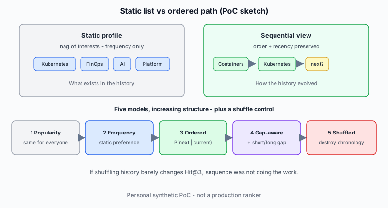
Recommendation does not have to be framed only as which item is most relevant to this user? It can also be framed as given the path this user has taken so far, what is most likely to be useful next?
That sounds like a small change in wording. It is not. Order changes meaning.
The PoC deliberately avoids Transformers at first. It compares five progressively more informed models:
- Global popularity - what is popular across everyone?
- Personal frequency - what has this user historically consumed most?
- Ordered transition - given the latest topic, what usually comes next?
- Gap-aware sequential - given the latest topic and the elapsed time, what usually comes next?
- Shuffled-order control - what happens if I intentionally destroy chronology?
The fifth model is the real test. If the sequential model performs equally well after I shuffle each user’s history, I have not proved that sequence matters.
What the data looks like
The dataset is synthetic by design. I generated 1,000 users and 26,020 timestamped interactions using a fixed seed, making repeated runs deterministic in my local implementation. Exact reproduction would also require publishing the generator and evaluation code.
Each event contains four fields: user_id, timestamp, topic, action.
Here is a sample journey for one generated user:
| Date | Topic | Action | What the sequence suggests |
|---|---|---|---|
| 2026-01-08 | Containers | View | Early infrastructure interest |
| 2026-01-13 | Kubernetes | View | Moves deeper into orchestration |
| 2026-01-31 | Kubernetes | View | Reinforces the topic |
| 2026-02-05 | Platform Engineering | View | Broadens from technology to practice |
| 2026-02-06 | Kubernetes | View | Revisits a prerequisite |
| 2026-02-09 | Platform Engineering | Like | Stronger intent signal |
| 2026-02-10 | Internal Developer Platforms | View | Natural adjacent topic |
| 2026-02-13 | Platform Engineering | Save | High-interest action |
| 2026-02-17 | Internal Developer Platforms | View | Continues the journey |
| 2026-02-20 | Developer Experience | View | Moves toward the outcome of platform engineering |
| 2026-03-11 | Python | Save | Long gap, then a different local direction |
A static model sees a collection of topics and frequencies. A sequence-aware model sees something closer to a journey. The March 11 Python event also shows why time may matter: a transition after one day may mean “continue the current task”; a transition after three weeks may mean “the user has returned with a new goal.”
Why synthetic data? I do not have a clean, large, publishable history of my own reading. Pretending that I do would make the story sound more personal and the experiment less honest. Synthetic data is appropriate for demonstrating the mechanism, evaluation design, and failure modes. It is not evidence that real users will produce the same gains.
How the journeys were generated
The generator contains several plausible technical learning paths. One runs Cloud Fundamentals -> Containers -> Kubernetes -> Platform Engineering -> Internal Developer Platforms -> Developer Experience -> FinOps. Another runs Python -> Data Engineering -> Embeddings -> Recommender Systems -> Sequential Recommendation -> LLM Ranking -> Evaluation.
Users do not move perfectly from left to right. The generator allows repetition, revisiting earlier concepts, skipping ahead, exploration, and longer gaps. A perfectly deterministic sequence would make the experiment trivial.
Evaluation: hide the future
For every user, interactions are sorted chronologically. The last event is held out as the test target. If the history is A -> B -> C -> D -> E, the model receives A -> B -> C -> D and must rank E as highly as possible. For the gap-aware model, the held-out event’s timestamp represents the simulated recommendation-request time; the held-out topic and action remain hidden.
I use Hit@3 as the primary metric: is the true next topic in the model’s top three predictions? I also report MRR@3 and NDCG@3. This is a per-user chronological split, not a global temporal cutoff. It prevents future events from the same user entering that user’s training history, but it does not model catalogue-wide changes over calendar time.
Five models
1. Global popularity recommends the same most-popular topics to everyone. Intentionally simple, and useful: a recommender that cannot beat popularity has not yet earned its complexity.
2. Personal frequency knows the user, but not the order of the user’s history. It asks what topics this person has interacted with most often. That is a traditional static preference profile.
3. Ordered transitions preserve chronology. For every adjacent pair of topics in the training histories, the model counts transitions and estimates P(next_topic = j | current_topic = i). A first-order Markov recommender:
for user in users:
    history = sort_by_time(user.events)
    for current, nxt in adjacent_pairs(history):
        transitions[current][nxt] += 1
At prediction time, the current topic becomes the context. No embeddings. No GPU. No attention. That simplicity is intentional.
4. Gap-aware sequential adds a deliberately crude time signal. Each transition belongs to one of two buckets: short gap (<= 7 days) or long gap (> 7 days). The model therefore learns two versions of its transition patterns: P(next | current, short_gap) and P(next | current, long_gap).
If I read about Kubernetes yesterday, platform engineering may be the natural continuation. If my last Kubernetes interaction was two months ago, the next topic may be driven more by a new goal than by the old session.
gap_days = (next_time - current_time).days
bucket = "short" if gap_days <= 7 else "long"
transitions[bucket][current][next_topic] += 1
This is not sophisticated temporal modeling. It is a probe: does time add any signal at all?
5. Shuffled-order control keeps the same topics but shuffles their order before learning transitions. The resulting model still knows which topics co-occur in similar users. What it loses is the actual journey. If performance barely changes, chronology was not doing much work.
Results
The deterministic run uses seed 42 and evaluates 1,000 held-out next events.
| Model | Hit@3 | MRR@3 | NDCG@3 | 95% bootstrap CI for Hit@3 |
|---|---|---|---|---|
| Global popularity | 0.560 | 0.455 | 0.482 | 0.529–0.590 |
| Personal frequency | 0.670 | 0.556 | 0.585 | 0.640–0.700 |
| Ordered transition | 0.794 | 0.684 | 0.712 | 0.768–0.819 |
| Gap-aware sequential | 0.819 | 0.693 | 0.725 | 0.795–0.842 |
| Shuffled-order control | 0.655 | 0.561 | 0.585 | 0.626–0.684 |
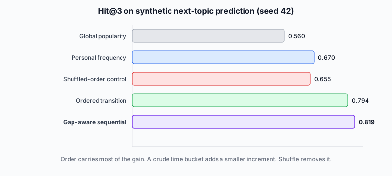
The absolute numbers are less important than the controlled differences.
Static preference -> sequence. Moving from personal frequency to ordered transitions increases Hit@3 from 0.670 to 0.794: +12.4 percentage points. The paired bootstrap 95% CI for the improvement is about +9.4 to +15.6 points. Inside this synthetic environment, knowing what tends to follow what adds substantial information beyond knowing what the user tends to like.
Sequence -> sequence + time. Adding the short/long gap feature increases Hit@3 from 0.794 to 0.819: another +2.5 percentage points (paired 95% CI about +1.2 to +3.8). That prevents an exaggerated conclusion. The experiment does not say that time is the dominant factor. It says:
Order carries most of the gain. A crude time signal adds a smaller incremental gain.
That is a more interesting result than forcing the article to support a “time-aware AI changes everything” headline.
The strongest evidence: shuffle the history
The gap-aware sequential model achieves Hit@3 = 0.819. The shuffled-order control achieves 0.655. The difference is +16.4 percentage points (95% CI: +13.5 to +19.3).
The shuffled model is not useless. Related topics still co-occur in the same users, so it retains some signal. But when chronology is destroyed, a large amount of predictive power disappears. That is the core finding of this PoC.
A concrete time-aware example
One generated user had this recent history:
| Date | Topic | Action |
|---|---|---|
| 2026-02-14 | FinOps | View |
| 2026-02-15 | FinOps | Save |
| 2026-02-18 | Cost Optimization | View |
| 2026-02-22 | Cost Optimization | Like |
| 2026-02-25 | Autoscaling | View |
| 2026-03-01 | FinOps | Save |
| 2026-03-07 | FinOps | Like |
| 2026-03-10 | Cost Optimization | View |
| 2026-03-24 | Observability | Save - held-out target |
Notice the 14-day gap before the held-out target.
Personal frequency and ordinary transitions both ranked FinOps, Cost Optimization, Autoscaling. The gap-aware model ranked FinOps, SLOs, Observability. It still did not rank the correct topic first, but it moved it into the top three.
That is the kind of behavior the time feature is intended to capture: after a longer break, the local transition pattern can differ from the immediate-session pattern. One example does not prove the model is generally better. The aggregate evaluation above is what matters. The example makes the mechanism easier to see.
Why not a Transformer first
It would have been easy to build a tiny SASRec-style model and make this article look more advanced. That would have weakened the experiment. Before adding a high-capacity architecture, I want to know whether simple signals already explain most of the result.
This question is especially relevant now. A 2026 Spotify Research paper, Do Sequential Recommendation Benchmarks Really Require Higher-Order Sequence Modelling?, evaluates strong recency-weighted pairwise methods against Transformer-based sequential recommenders. On several commonly used benchmarks, the simpler probes match or outperform reproduced Transformer baselines. MovieLens-20M is a clear exception, where the Transformer retains a substantial lead.
The lesson is not “Transformers are unnecessary.”
The lesson is:
A complex model should have to beat strong simple baselines that already capture popularity, recency, and pairwise transitions.
That is why this PoC begins with a Markov-style transition model rather than a neural network. If a future Transformer beats it materially on the same chronological evaluation, then we have evidence that higher-order context contributes something real.
What this PoC shows - and what it does not
What it demonstrates. Within the generated dataset: a static personal profile beats global popularity; preserving chronology beats the static profile; adding a simple elapsed-time feature improves the sequential model slightly; destroying chronology significantly reduces performance.
That means the setup isolates three different kinds of signal: preference, plus sequence, plus time.
What it does not prove. The dataset deliberately contains sequential structure. A sequence-aware model should discover it. The measured gains - 12.4 points, 16.4 points, or any other number - must not be presented as expected production uplift.
Real recommendation systems are harder: users have multiple simultaneous interests; items are dynamic and often new; actions have different intent strengths; candidate retrieval and ranking are separate problems; relevance is only one objective. Diversity, freshness, safety, creator quality, fairness, and long-term value also matter. Offline metrics do not guarantee online product gains.
The honest conclusion is narrower:
The PoC demonstrates a method for testing whether chronology and time carry predictive signal. The next step is to run the same ablation on real interaction logs.
From PoC to a real architecture
A production system would be much larger than this experiment, but the conceptual layers remain understandable:
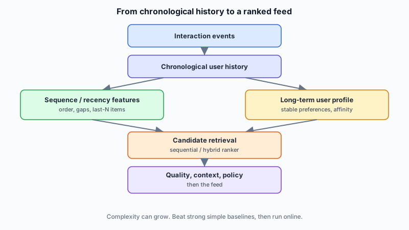
At small scale, the “sequential ranker” could literally be the transition model used here. At large scale, that component might become a Transformer or another history encoder. The long-term profile, context features, policy rules, and product objectives can then be fused into the final ranking decision.
The architecture can become complex. The measurement principle should remain simple:
Does the new model beat strong static, recency, and transition baselines on chronological offline evaluation - and then survive an online experiment?
What I would build next
The next step should not be “add more layers.” I would proceed in this order:
- Replace synthetic histories with real chronological events
- Weight actions differently: view, then like, then save
- Use several recent history items with recency decay
- Add context such as device, session, or time of day if relevant
- Build a SASRec-style or Transformer model
- Compare it against the strongest simple sequential baseline
- Only then consider production serving and online testing
The third step is particularly important. Instead of conditioning only on the latest topic, a stronger non-neural model can aggregate evidence from several recent interactions:
score(candidate) =
    w1 * P(candidate | last_item)
  + w2 * P(candidate | item_before_last)
  + w3 * P(candidate | older_item)

w1 > w2 > w3
That produces a much stronger test for whether a Transformer is learning genuine higher-order structure rather than simply reproducing recency-weighted pairwise statistics.
Closing
I started this experiment because of an LLM discussion. The useful lesson is not really about LLMs. It is about representation.
A user profile represented as {Kubernetes, AI, FinOps, Platform Engineering} is not equivalent to Kubernetes -> Platform Engineering -> Developer Experience -> FinOps. The first says what exists in the history. The second also says how the history evolved. When timestamps are included, we can begin to distinguish an active journey from an old preference.
The sentence I would keep from this entire PoC:
A user’s history is not only a list of preferences. It is an ordered path through changing intent.
The experiment is still small and synthetic. That is fine. A PoC should not pretend to be production evidence. What it gives me is something more useful than a copied architecture: a falsifiable method.
Preserve the sequence. Measure it. Destroy the sequence. Measure again. Add time. Measure again. Then increase model complexity only when the data justifies it.
That is the part I would carry into a real recommendation system.
References
- Software Engineering Daily, How LLMs Are Reshaping Recommendation Systems, 18 August 2026
- Hertel et al., An Industrial-Scale Sequential Recommender for LinkedIn Feed Ranking, arXiv:2602.12354, 2026
- Petrov et al., Do Sequential Recommendation Benchmarks Really Require Higher-Order Sequence Modelling?, arXiv:2608.19833, 2026
- Spotify Research, sequential-capacity-probes
PoC details: 1,000 synthetic users, 26,020 interactions, chronological leave-last-event-out evaluation, seed 42, Hit@3 / MRR@3 / NDCG@3, and bootstrap confidence intervals. The data and results are synthetic and should be interpreted as a demonstration of methodology rather than expected production uplift.
This is a personal blog. The views, thoughts, and opinions expressed here are my own and do not represent, reflect, or constitute the views, policies, or positions of any employer, university, client, or organization I am associated with or have been associated with.